
89. Python Calculus Basics#
89.1. Introduction#
Calculus is the foundation of modern mathematics. As long as it is a machine learning algorithm, formula derivation is necessary. As long as formula derivation is carried out, calculus must be used. This experiment first explains the basic knowledge of calculus, then elaborates on the principles of the gradient descent algorithm and the least squares method in detail. Finally, these algorithms are used to complete a simple optimization problem. This experiment attempts to explain the knowledge related to calculus in a simple way, and each knowledge point is accompanied by relevant examples. These examples are simple but can well reflect the relevant concepts. Therefore, I hope you can calm down and read and study it carefully.
89.2. Knowledge Points#
Linear Functions and Nonlinear Functions
Derivatives and Partial Derivatives
Chain Rule
Gradient Descent Algorithm
Local Optimum and Global Optimum
Least Squares Method
Functions are one of the most important theories in basic mathematics. We probably started learning about functions and their basic properties at a very young age. Therefore, we will not explain the properties that we are already very familiar with here, but only elaborate on the function knowledge related to machine learning.
89.3. Linearity and Nonlinearity of Functions#
A function represents the mapping relationship from one variable to another.
If this relationship is a linear function, we call it a linear relationship (also known as a linear function). More通俗地讲, if two variables are used as the abscissa and ordinate of a point respectively, and its graph is a straight line on the plane, it indicates that the relationship between these two variables is a linear relationship. On the contrary, if the graph is not a straight line, then this relationship is called a nonlinear relationship, such as exponential functions, logarithmic functions, power functions, etc.
Similarly, in machine learning, we generally call the problems that can be solved using linear functions linear problems, and the problems that must be solved using non-linear functions non-linear problems. Take the classification problem as an example, as shown in the following figure:

For Figure 1, the problem where we can use a straight line to classify data is a linear problem, and we call the function where this straight line lies a linear classifier. Similarly, for a problem like Figure 2 that requires using a curve to complete classification, we call it a non-linear problem, and this curve is also called a non-linear classifier.
89.4. Derivative#
The function value changes as the independent variable changes, and the rate of this change is the derivative. The derivative of the function \(f(x)\) can be denoted as \(f'(x)\) or \(\frac{df}{dx}\). What the derivative measures is actually the influencing ability of a variable on the function value.
The larger the derivative value, the greater the impact of each unit change in this variable on the final function value. When the derivative value is positive, it means that the function value increases as the independent variable increases. On the contrary, if the derivative value is negative, it means that the function value decreases as the independent variable increases.
The common functions and their corresponding derivatives are as follows:
|
Original function \(f\) |
Derivative function \(f'\) |
|---|---|
Any constant |
0 |
|
\(x\) |
1 |
|
\(e ^ { x }\) |
\(e ^ { x }\) |
|
\(x ^ { 2 }\) |
2\(x\) |
|
\(\frac { 1 } { x }\) |
\(\frac { - 1 } { x ^ { 2 } }\) |
|
\(\ln ( x )\) |
\(\frac { 1 } { x }\) |
89.5. Partial Derivative#
The functions we listed above have only one independent variable. What if there are multiple independent variables? How do we find the derivative?
For example, for the function \(f = x + y\), how can we measure the influence of \(x\) and \(y\) on the function value \(f\) respectively? To solve this problem, the concept of partial derivative is introduced in mathematics.
For a multivariable function \(f\), finding the partial derivative of \(f\) with respect to one of its independent variables \(x\) is quite simple. It is to regard the other independent variables that are not related to \(x\) as constants, and then perform single-variable differentiation. What is obtained is the partial derivative of \(f\) with respect to \(x\). For example:
If there is a function \(f = x + 2y\), then the result of taking the partial derivative of \(f\) with respect to \(x\) is \(\frac{\partial f}{\partial x}=1\), and the result of taking the partial derivative of \(f\) with respect to \(y\) is \(\frac{\partial f}{\partial y}=2\).
If there is a function \(f = x^2 + 2xy + y^2\), then the result of taking the partial derivative of \(f\) with respect to \(x\) is \(\frac{\partial f}{\partial x}=2x + 2y+0\), and the result of taking the partial derivative of \(f\) with respect to \(y\) is \(\frac{\partial f}{\partial y}=0 + 2x + 2y\).
89.6. Gradient#
As we mentioned before, for a single-variable function, the sign of the derivative value represents the “direction” of the influence of the independent variable on the function value: increasing or decreasing.
So for a multi-variable function, how can we express the direction of the change in the function value? This introduces the concept of the gradient. The direction represented by the gradient is actually the direction in which the function value \(f\) increases most rapidly.
The gradient is a vector, and the length of the vector is equal to the number of independent variables. The gradient is a vector composed of the partial derivative values corresponding to each independent variable. For example, the gradient vector of \(f(x, y, z)\) is \((\frac{\partial f}{\partial x}, \frac{\partial f}{\partial y}, \frac{\partial f}{\partial z})\).
For the function \(f = x^2 + 2xy + y^2\), its gradient vector is \((2x + 2y, 2x + 2y)\). For specific values of the independent variables, such as the point where \(x = 1\) and \(y = 1\), its gradient vector is \((4, 4)\). Another example is the point where \(x = 10\) and \(y = -20\), and its gradient vector is \((-20, -20)\).
We can understand the gradient (the combination of partial derivatives of each variable) in a multi-variable function as the derivative in a single-variable function.
89.7. Chain Rule#
Deriving or finding partial derivatives of “simple functions” like the ones above is relatively straightforward. However, for finding derivatives of “composite functions”, some new knowledge is required. For example, functions like the following:
For the derivative of the composite function \(y\) with respect to \(x\), we can use the chain rule of differentiation.
The form of the chain rule is as follows:
We first regard \(g(x)\) as a whole and denote it as \(u\). So the expression can be transformed into \(y = f(u)=\frac{1}{u}\), and then we get:
Since $\(u = e ^ { x }\)\(, then: \)\(\frac{du}{dx}=e^x\)$
Then according to the chain rule, we can get:
This is the whole process of the chain rule. When dealing with composite functions, we first regard the inner function as a whole, take the derivative of the outer function, and then take the derivative of the inner function. This process of taking the derivative of the function of the current layer layer by layer like peeling an onion and finally multiplying all the derivatives to obtain the derivative of the composite function is called the chain rule. The chain rule is mainly used in the backpropagation of neural networks.
89.8. Optimization Theory#
89.9. Objective Function#
Simply put, the objective function is the goal of the entire problem. In machine learning, we often take the distance between the predicted value and the true value as our objective function. The smaller this function is, the higher the prediction accuracy of our model is proven.
Model training is actually a process of using relevant algorithms to find the minimum value of the objective function.
To facilitate the explanation, we can introduce a simple linear programming problem: A 20-meter-long iron wire is cut into two sections, which are then bent into two squares respectively. To minimize the sum of the areas of the two squares, what are the lengths of the two sections of the iron wire?
Let one section be of length \(x\), then the other section is of length \((20 - x)\). Then, based on the above description, we can define the objective function of this problem as follows:
The above function \(y\) is the objective function of the entire problem. Our goal is to find the minimum value of \(y\) and the value of \(x\) corresponding to the minimum value.
We can use Python to define the function \(y\) as follows:
import math


def obj_fun(x):
    s1 = math.pow(x/4, 2)
    s2 = math.pow((20-x)/4, 2)
    return s1+s2
obj_fun(x=5)
15.625
As above, we defined our objective function
obj_fun, which can calculate the value of
\(y\)
corresponding to any
\(x\)
according to the above formula. After obtaining the
objective function, next we need to find the minimum value
of this function. So how do we find the minimum value of
this function? Here we use the gradient descent algorithm.
89.10. Gradient Descent Algorithm#
Since the above problem is only a univariate function problem, we can simply use the derivative rule of the function to directly find the minimum value of the above function. However, using the gradient descent algorithm to solve this problem is a bit of an overkill. But for a better introduction to this algorithm, we will use this relatively simple function as the objective function.
We can analogize the gradient descent algorithm to a process of going down a mountain. Suppose a person is trapped on a mountain and needs to quickly come down to the bottom of the mountain. However, due to thick fog in the mountain, the visibility is very low. As a result, we are unable to determine the path down the mountain and can only see some information around us. That is to say, we need to take one step, look around, take another step, and look around again. At this time, we can use the gradient descent algorithm as follows:
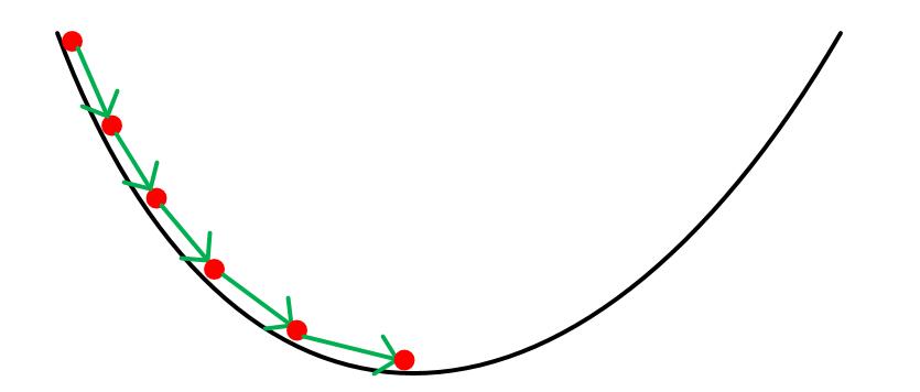
First, taking the current position as a reference, find the steepest direction around this position and take a step in that direction. Then, taking the new position as a reference, find the steepest direction again and take a step in that direction. Repeat this process until reaching the lowest point.
The objective function we need to find can also be regarded as a mountain, and our goal is to find the minimum value of this mountain, that is, the bottom of the mountain. The steepest direction mentioned above is also the direction in which the value of the objective function decreases fastest, which is the opposite direction of the gradient (the gradient direction is the direction in which the function value increases fastest).
Therefore, in order to find the minimum value of a function, we need to calculate the gradient using the current position and then update the position based on the gradient. Then, we find the gradient according to the current position and update again. Repeat this process until the function value is minimized. The mathematical expression for updating the next position based on the gradient and the current position is as follows:
The above formula shows the solution process for the minimum value of the function \(J(\theta)\).
Among them, \(\theta^0\) represents the current position, \(\theta^1\) represents the next position, \(\alpha\) represents the step size (i.e., the distance of one update), and \(-\triangledown J(\theta^0)\) represents the opposite direction of the gradient of \(\theta^0\).
For the convenience of calculation, here we use a univariate function as an example. Let the function \(J(\theta)=\theta^2\). Since the gradient of a univariate function is the derivative, so \(\triangledown J(\theta)=J'(\theta) = 2\theta\). Here, the step size is set to 0.4, and the starting point of gradient descent is \(\theta^0 = 1\). Next, we use gradient descent for iteration:
As shown above, after four calculations, the value of our \(J(\theta)\) is getting smaller and smaller. If we iterate thousands of times, then the value of \(J(\theta)\) will gradually approach the minimum value. Of course, it may never be equal to the minimum value, but it can get infinitely close to that value.
Next, let’s get back to solving for the minimum area of the two squares formed by the wire. The function is still as follows:
By calculation, the gradient of this function can be obtained as \(y' = \frac{x}{4}-\frac{5}{2}\).
Let’s write the code for the gradient function of this function:
def grad_fun(x):
    # y' = x/4-5/2
    return x/4-5/2
grad_fun(1)
-2.25
Next, let’s use the gradient descent algorithm to solve for the minimum value of y:
# 设置误差最小为 0.0001
# 即当函数下降距离已经小于 0.00000001 证明已经很接近最小值,无需继续迭代
e = 0.00000001
alpha = 1  # 设置步长
x = 1  # 设置初始位置
y0 = obj_fun(x)
ylists = [y0]
while(1):
    gx = grad_fun(x)
    # 梯度算法的核心公式
    x = x - alpha*gx
    y1 = obj_fun(x)
    ylists.append(y1)
    if(abs(y1-y0) < e):
        break
    y0 = y1
print("y 的最小值点", x)
print("y 的最小值", y1)
y 的最小值点 9.99971394602207
y 的最小值 12.50000001022836
From the above results, we can see that when \(x\approx10\), \(y\) obtains the minimum value of the function.
Next, let’s show the iterative process of \(y\):
import numpy as np
import matplotlib.pyplot as plt
%matplotlib inline

plt.title("loss")
plt.plot(np.array(ylists))
plt.show()

As shown in the figure above, we solved for the minimum value of the function y using the gradient descent algorithm. Of course, due to the step size issue, the result we found may not be exactly the same as the correct answer (it can only approach it infinitely). However, through this method, we can well find the minimum point of any complex function.
Next, let’s find the minimum value of a complex function \(f(x,y)= x^2+y^2-6x-4y+29\).
First, write the function \(f(x,y)\):
def func(x, y):
    return x**2+y**2-6*x-4*y+29
func(1, 1)
21
Next, write the function to calculate the gradient. Since there are two unknowns, the partial derivatives of the two variables need to be returned:
def grads(x, y):
    # 计算x的偏导
    dx = 2*x-6
    dy = 2*y-4
    return dx, dy
grads(1, 1)
(-4, -2)
Next, let’s use the gradient descent algorithm to calculate the minimum value of this function:
e = 0.00000001
alpha = 0.1
x = 1
y = 1
f0 = func(x, y)
flists = [f0]
while(1):
    dx, dy = grads(x, y)
    # 梯度算法的核心公式
    x = x - alpha*dx
    y = y - alpha*dy
    f1 = func(x, y)
    flists.append(f1)
    if(abs(f1-f0) < e):
        break
    f0 = f1
print(f"f 的最小值点:x={x},y={y}")
print(f"f 的最小值 {f1}")
f 的最小值点:x=2.999891109642585,y=1.9999455548212925
f 的最小值 16.000000014821385
According to the above results, we can obtain that when \(x\approx3\) and \(y\approx2\), the original function reaches its minimum.
89.11. Local Optimum and Global Optimum#
Of course, the gradient descent algorithm doesn’t always find the minimum value of a function, as shown below:
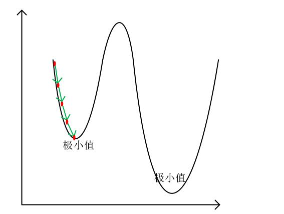
As can be seen from the above figure, we used gradient descent to find a local minimum point of the function, but did not find the true minimum point.
In fact, there are many such local minimum points in complex functions. We call this kind of local minimum point within a certain range the local optimum point, and call the minimum point among these local minimum points the global optimum point.
Therefore, in order to ensure that the point we find is as close as possible to the global optimum point, the setting of the step size in gradient descent is extremely crucial. We can set the step size slightly larger so that the algorithm can cross the “valleys” on both sides of the local minimum point and thus find the true minimum point. Of course, if the step size is set too large, it may also prevent us from finding the desired answer.
In fact, many machine learning problems are optimization problems of a very complex function. These functions often have a large number of extreme points and optimal points. Sometimes, it is really difficult for us to tell whether the point we find is the global optimum. Similarly, we also have no evidence to prove that our point is the minimum point (unless we list all the points using the exhaustive method).
In fact, in machine learning, most of the time, we can only try our best to adjust the parameters and find a relatively good local minimum point as the optimal point. In other words, most of the time, the solution of the model we train is actually just a local optimal solution.
This is like finding a partner. We can never guarantee that our current partner is the most suitable one for us. We just find a local optimal solution in the forest. But indeed, this solution is a good one among many solutions, and we should cherish him/her well.
89.12. Least Squares Method#
The least squares method is also one of the most commonly used theories in linear programming. This method is mainly used to fit data points. Simply put, it is to find a suitable data line (functional form) to represent the distribution of all data. Suppose we need to use this method to fit a univariate function problem, then we can describe the problem as follows:
Suppose there are (n) data points with coordinates ((x_1,y_1),(x_2,y_2),(x_3,y_3)\cdots(x_n,y_n)). We need to use the function (y = kx + b) to describe the functional relationship between the (y)-coordinates and (x)-coordinates of these data points. Here, we can use the least squares method to obtain the specific values of (k) and (b).
First, let’s simulate these data sets. Assume that these data sets are random numbers between (y = 2x+3+(-1,1)).
x = [0]
y = [3]
for i in range(60):
    xi = np.random.rand()*5
    yi = 2*xi+3 + np.random.rand()*(-1)
    x.append(xi)
    y.append(yi)
plt.plot(x, y, '.')
[<matplotlib.lines.Line2D at 0x1178e7cd0>]

As shown in the figure above, we need to find a straight line (y = kx + b) to measure the distribution of all the data.
So what kind of straight line can best represent the data distribution? Of course, if all the data points can fall on the straight line, then this straight line is definitely the best one. However, in real life, there won’t be such ideal data. Generally, the data distribution will be like the figure above, showing a trend but not coinciding with the straight line.
For such actual data points, how should we find a straight line that best reflects the distribution? The least squares method gives the answer. The core idea of this algorithm is to “minimize the sum of squared errors”. That is to say, if the straight line (y = kx + b) we find has the minimum sum of distances from all data points, then this straight line is the best fit line.
The definition of the sum of squared errors is as follows:
According to the extreme value theorem, when \(f\) takes the minimum or minimum value, the slope of the point corresponding to \(f\) must be 0, that is, the derivative of the unknown is 0. Since \(k\) and \(b\) are unknowns at this time, the partial derivatives of \(f\) with respect to \(k\) and \(b\) should be 0. As follows:
Let’s expand the brackets to get:
Assume that \(A=\sum_{i = 1}^n(x_i^2)\), \(B = \sum_{i = 1}^n(x_i)\), \(C=\sum_{i = 1}^n(x_iy_i)\), \(D=\sum_{i = 1}^n(y_i)\), then the above equations can be substituted as:
Solving the above system of binary equations gives:
Since the data points are known, we can easily calculate the specific values of \(k\) and \(b\) according to the above formulas.
The above entire process is the whole process of the least squares method. First, we need to determine the form of the function that describes the data set. Then, based on the function and the data set, we obtain the formula for the sum of squared errors. Finally, we use the least squares method to find the specific values of each parameter in the formula.
Let’s use the least squares method to fit the simulated data above and observe the differences between the predicted values of \(k\) and \(b\) and the true values:
A = np.sum(np.multiply(x, x))
B = np.sum(x)
C = np.sum(np.multiply(x, y))
D = np.sum(y)
n = len(x)
k = (C*n-B*D)/(A*n-B*B)
b = (A*D-C*B)/(A*n-B*B)
print("实际的 k=2,b=3")
print("利用最小二乘法得到的 k = {},b={}".format(k, b))
实际的 k=2,b=3
利用最小二乘法得到的 k = 1.9970925836606068,b=2.469418590058912
Of course, the above only uses the least squares method to fit a relatively simple unary function. The least squares method can also produce good results when fitting complex multivariate functions. However, since the derivation of the formula is relatively complex, it will not be demonstrated here. If you are interested, you can try to find the specific values of each coefficient using the least squares method and data points when the form of the original function is assumed to be \(y = k_1x^2 + k_2x + b\).
89.13. Summary#
The gradient descent algorithm is one of the most widely used optimization and solution methods in machine learning. For the convenience of explanation, the examples cited in this experiment are relatively simple. If you want to understand this algorithm more thoroughly, you can try to learn the relevant knowledge of artificial neural networks to further understand the advanced applications of the gradient descent algorithm.